It’s always a challenge to make a quality estimation of inputs to the valuation model like the one utilized in the Startup Valuator. If your company plans to acquire venture capital you should be ready to get the most adequate information about the market. That’s a topical problem for emerging market segments with low entry barriers and high rates of business failures. And e-commerce is a good example.
There is no better way to prove that your company worth the value you expect than using the method of comparables. But multipliers are not always available or they aggregate the information, which is hardly relevant. That’s why I recommend you to use a DCF approach as a backup. Use Startup Valuator with the parameters estimated carefully and you’ll get a lot of useful information on the value of your company.
This post will be about the estimation of growth during the post forecasted period. This parameter is extremely important for the reason that it’s used in calculation of terminal value. For the most of internet companies terminal value has the biggest share to the total value of the firm due to the high expectation of future growth and low need in capital consuming production facilities.
My idea is that we can say for sure what this parameter will be. We will need the following instruments: Microsoft Excel or some soft similar to that and NLREG. The last program is an awesome thing for nonlinear regression analysis.
Let me say again, that our goal is to calculate g (future market growth) and be as much realistic as we can. That’s quite challenging, but we’ll make a try.
We are taking a Russian internet company which conducts its’ operations in the segment of context advertising aggregators. It’s good for you to know what the revenue is. The data is presented by months on the graph below:
What drives the revenue change in a way like this? There is no sophisticated answer. It’s clear that the more people are surfing the web the more the probability of their accurance on the website of the company. Let’s see if our assumption is adequate.
Both variables are growing in their value. We’ll gather more information by taking the first derivative of them. Look at the example in this google spreadshit. My results are the following:
The founding is not trivial. We have almost proved that our assumption is down to earth. There is some sort of correlation between these two factors. It’s not linear. Next we’ll use some econometrics. To figure out what sort of dependence there is we build a correlation pole. The correlation pole allows conducting the interpolation, which is a crucial point of the analysis in our case.
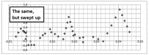
Hm… That’s not as good as I expected. Human being is still much cleverer than any algorithm, so we’ll help the computer a little to make a more quality estimation.
Now it’s a whole new ball game! I can’t help thinking that these stuff is very similar to a sine wave with a linear trend:
So we download the demo of NLREG and type into the following command:
Variables RIU,Revenue;
Parameters p0,p1,Amplitude,Period=2.3,Phase=0;
Function Y = p0 + p1*X + Amplitude*sin(2*pi*(X-Phase)/Period);
Plot Residual,Grid;
Data;
[data array]
I won’t publish here the full report. The most important thing for us is that p-value for all the parameters except p0 is less then 0.001. That’s very good!


No comments:
Post a Comment